Introduction
At the beginning of this section, I would like to apologize for a long time there was no news - I’ll try to catch up in the coming weeks :-) . Below is a link to the answers to the exercises in the previous section. I encourage you to verify your answers.
Homework
1. The triangle will be drawn correctly, but will be enlarged so that its vertices will “come out” of the scope of OpenGL’s window.
2. The image must be zoomed out twice, so the last two parameters in our viewport has respectively width: width/2 and height: height/2, where width and height are the width and height of our OpenGL’s window.
Then we need to set the viewport on the center of the screen. So the bottom left corner of the viewport must be in 1/4 width and 1/4 height of the OpenGL window (remember that the bottom left corner of the OpenGL window is the point (0, 0)). Thus, the first two parameters have the values: width/4 and height/4.
glViewport(width/4, height/4, width/2, height/2);
3. To draw a square, you have to use two triangles. To this end, we update the array vertices with new values:
glm::vec3 vertices[] = { glm::vec3(-1.0f, -1.0f, 0.0f),
                         glm::vec3(-1.0f,  1.0f, 0.0f),
                         glm::vec3( 1.0f, -1.0f, 0.0f),
                         glm::vec3(-1.0f,  1.0f, 0.0f),
                         glm::vec3( 1.0f,  1.0f, 0.0f),
                         glm::vec3( 1.0f, -1.0f, 0.0f) };
And change the last parameter in the glDrawArrays(), which shows how many vertices of the array you want to draw (in this case 6 - two triangles; two points are repeated - avoiding the redundancy will be discussed in the following sections of this course).
glDrawArrays(GL_TRIANGLES, 0, 6);
In this part of the course will only be the theory as to how the whole rendering process runs in OpenGL - it will be the introduction to shader programs as well. I think that it’s quite an important aspect while learning 3D graphics programming, as it allows to understand the behavior of OpenGL and we will be more aware of what is happening behind the “scenes” when we want to draw a virtual scene on the screen. In addition, this knowledge will help us to understand how shaders work so we can easily “color” our triangle and transform it.
Programmable rendering pipeline
Long, long ago, when OpenGL 1.0 was on top, in graphics cards was implemented so called fixed rendering pipeline. Its advantage was that the little time was needed to draw a triangle on the screen, color it and rotate freely. More specifically, developers were limited only to use the “building blocks” that someone had implemented to create something new.
Such an approach was good up to a point where the capabilities of these “bricks” got exhausted and developers wanted to create something new, unique, faster. Therefore, graphics card manufacturers have invented programmable rendering pipeline, in which at certain stages of drawing geometry, a programmer might be able to affect (by writing shader programs) how the geometry will look like (operations on vertices) and how it will be colored (operations on pixels/fragments). With successive versions of OpenGL, it became possible to affect more and more individual rendering stages and began to deviate from obsolete, fixed rendering pipeline. The modern rendering process is shown in the following picture:
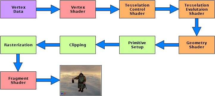
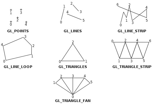
As you can see from the above diagram, we start by transferring primitives’ vertices that we want to draw. Primitive is the basic geometric figure, which we can draw. OpenGL offers us primitives such as points (GL_POINTS), lines (GL_LINES), line strips (GL_LINE_STRIP), line loops (GL_LINE_LOOP), triangles (GL_TRIANGLES), triangle strips (GL_TRIANGLE_STRIP), triangle fans (GL_TRIANGLE_FAN). Below is a picture of the previously mentioned geometric primitives:
Then the vertex shader is processing these data that transforms vertices from the local coordinate system of the object to the screen coordinates (more about transformations will be in the following tutorials); Tessellation shader that actually consists of two separate programs and Geometry Shader (more on Tessellation and Geometry shaders will be in the following tutorials). Then, primitives are created which are then “cut” if they come out of the visibility of virtual “eye” (camera). At the end, the fragment shader is run, which colors the pixels/fragments. After this, different tests are run (scissor test, alpha, stencil test, depth, blending) and finally we get rendered 3D scene.
In the following sections we will look closely at each of these steps to find out what each of them is exactly doing.
Vertex Data
At the beginning we prepare our data, which show some form, for instance triangle and place them in corresponding array (array vertices from the previous part of this tutorial). When we prepared the vertices, they must be sent to the OpenGL object that can store the data - buffer. Sending data to the buffer OpenGL is done by calling the function glBuferData(). When the data is in the cache, we can draw it by calling glDrawArrays(). Drawing means the transmission of the data further to rendering pipeline.
Vertex Shader
The next process, which gets data after expressing a desire to draw is Vertex Shader. It is a process over which we have full control and we define it ourselves. It is required to implement and use at least one vertex shader when we want to use OpenGL in a modern manner.
Vertex Shader is a simple program that we write and is called for each vertex, we want to draw. Its main objective is to convert the coordinates of the vertices to the screen coordinates, but it also can be used, for example to transform the position of these vertices.
Tessellation Control & Evaluation Shader
Now the data is on stage of Tessellation Control Shader and Tessellation Evaluation Shader. They are similar to Vertex Shader, over which we have full control. They are not mandatory as they are used for special purposes. Unlike the Vertex Shader, Tessellation shaders work on patches. Generally they are used for tessellating geometry - increase the number of primitives in the geometric shape in order to obtain smoother mesh of a model.
Geometry Shader
The next process, which gets the data is Geometry Shader. It is, like Tessellation shader, not compulsory stage (you can but you do not have to write it) and is used for additional processing of geometry (transmitted data), for example to create new geometric primitives before rasterization.
Primitive Setup
Earlier stages operated only on the vertices that had to create the appropriate geometric primitives. In this step, the geometric shapes are created on the basis of these vertices, which have been previously processed (or not).
Clipping
Sometimes it may happen that the vertices can be placed outside the viewport - an area where we can draw - a geometrical figure is partially in the viewport, and partly outside it. To this end, vertices that lie outside the viewport, are modified in such a way that none of them was not outside the viewport.
If the figure is entirely in the viewport, its vertices are not modified, and if it lies completely outside the viewport those vertices will not be included in the next steps - they will be rejected.
This is an automatic process - OpenGL deals with it itself.
Rasterization
Then, primitives are sent to the rasterizer. Its task is to determine which pixels of the viewport are covered by a geometric primitive. In this stage fragments are generated that is information about the position of the pixel and interpolated vertex color and texture coordinate.
Two successive stages deal with processing of these fragments.
Fragment Shader
Just as the vertex shader, this is the stage over which we have full control and is mandatory to define (because how OpenGL has to know how to paint the geometry?). At this stage, fragment shader is performs operations once for each fragment from the rasterization process. In this process, we can define the final color (whether defined by a programmer or computed from the calculations of light) and sometimes fragment depth value. Instead of the usual color, we can apply a texture on the fragment to make our 3D scene more realistic.
Fragment Shader can also stop processing of the fragment if it should not be drawn.
The difference between the Vertex (including Tessellation and Geometry shaders), and the fragment shader is that the Vertex Shader positions and transforms the primitive on the scene, and the fragment shader gives a color to the fragment.
Post Fragment Shader operations
Additionally, after the operations that we define ourselves in the fragment shader, are made final actions on particular fragments. These additional steps are described in the following sections.
Scissor test
In the application, we can define a rectangle which will limit the scope of the rendering. Each fragment, which is outside the defined area will not be rendered.
Alpha test
After the scissor test, it is time for alpha test. It is used to determine the transparency of the specific fragment. This test compares the alpha value of the fragment and the value that was defined in the program. Then the relationship between these values is being examined (if its larger, smaller, equal to, and so on) which makes the test to pass. If the relationship does not pass the test, the fragment is discarded.
Stencil test
Another test is a test template that reads the value of the stencil buffer in the position of the specific fragment and compares them with the values defined by the application. Stencil test passes only if the corresponding relationship is satisfied (the value is equal to, greater than, less than, etc.). Otherwise, the test fails, and the fragment is discarded.
In this case, we can define what happens in the stencil buffer if the test is successful (it is used in one shadow rendering technique which will be shown in the following parts of this tutorial).
Depth test
Depth test compares the depth of the fragment with the depth that is in a depth buffer. When the fragment depth does not satisfy the relationship (which is specified in the application) with the value in the depth buffer, the fragment is rejected. By default, this relationship is set to “less than or equal to” in OpenGL, but we can change it. So if the fragment depth value is less than or equal to the value of the depth buffer, the buffer is replaced with the value of the depth of this fragment.
This is an important test that allows us to hide one object after another.
Blending
When all tests are completed, the color of the fragment is mixed with the color in the image buffer. The color value of the fragment is combined with the color in the image buffer (or the color of a fragment can replace the value in the image buffer). This step may be configured to obtain the transparency effect.
That’s all. Congratulations to the hardy ones who have come to the end of this article and deepen their knowledge. If you do not understand everything at this stage - do not worry! All will become clear in the following sections of this course, where I hope, will be only practical lessons. In the next lesson we will write the first shader.
References
- OpenGL 4.4 documentation
- Mathematics for 3D Game Programming and Computer Graphics, Lengyel Eric, 2012
- Real-Time Rendering Third Edition, Akenine-Moller T., Haines E., Hoffman N., 2008